
Michael Rich
Midterm Analysis Report
Types of Risk Measurements Chosen and their Properties
Types of Risk Exposures:
I chose to analyze and measure three different risk categories that would be found within S&P 500 firms.
- Supply Dependence Risk (Risk associated with the dependence on the supply of certain materials/products/labor that are needed for the firm to sufficiently run their business operations. Such disruption in supply or supply chain can significantly impact the firms economic standing.)
- Competitor Based Risk (Risk associated with firms that face intense competition.)
- Regulatory/Political Based Risk (Risk associated with political or regulatory changes such as decisions made by the government regarding taxes, laws, and spending. I used three different variations to measure this risk.)
How the Risk Exposures were measured:
I used textual analysis to measure these risks. I first downloaded the annual reports (10K’s) of all of the current S&P 500 companies (this is done in download_text_files.ipynb). Then, I extracted the text from each 10K report and used regular expressions to count how many times certain words appeared next to eachother within the text. With a higher the count, that would imply that the given risk would be higher for that particular firm. (this is done in measure_risk.ipynb)
For example, in measuring the Supply Dependence Risk, I used the following regular expression:
(['(supply|supplies|supplier|logistics|labor)','(risk|harm|adverse|negative|cost|suffer)'],15)This expression finds words such as “supply” and “labor” and if they are near any of the words such as “risk” and “adverse” (within 15 words), then that would add one to the total risk exposure of that firm.
The following expressions were used in determining the other risk factors:
| Risk Factor | Word group 1 | Word group 2 | Max num words between groups |
|---|---|---|---|
| Competitor Based Risk | competitor,competition,competitive,position,customer | risk,harm,factor,adverse | 15 |
| Regulatory/Political Based Risk (1) | government,regulation,FDA,law,politic,compliance | risk,harm,cost,time,liability,adverse | 15 |
| Regulatory/Political Based Risk (2) | government,regulation,FDA,law,politic,compliance | risk,harm,cost,time,liability,adverse | 7 |
| Regulatory/Political Based Risk (3) | regulat,SEC,politic,international,tax | harm,negativ,adverse,decreas,susceptible | 15 |
Reasoning For Chosen Risks:
-
Supply Dependence Risk
Supply chain was a large issue at the beginning of the covid outbreak. There are several firms that are more reliant on the supply of materials, labor, and other factors. I chose to measure this risk specifically because I wanted to see if there would be data to support my hypothesis that there would be lower returns for firms that depend on supply chain during the start of a pandemic-like outbreak. -
Competitor Based Risk
Almost all firms have competition, but some face more competition than others. I chose to measure this type of risk because I was interested in learning how competition within different industries and firms affected returns during economic downturn. -
Regulatory/Political Risk
Regulatory issues is something most firms have to deal with, and come covid came an onslaught of new regulations such as mask mandates and policy controls. I was interested in capturing correlations that could suggest that firms with a higher exposure to this risk were negatively affected regarding their returns when covid started.
Statistical Properties:
The following code will output a summary of statistical properties regarding the risk measurements.
#Load output/sp500_accting_plus_textrisks.csv file
import seaborn as sns
import pandas as pd
from statsmodels.formula.api import ols as sm_ols

sample_csv = "output/sp500_accting_plus_textrisks.csv"
sample_firms_risks = pd.read_csv(sample_csv)

sample_firms_risks = sample_firms_risks.drop(['Unnamed: 0'], axis=1)

sample_firms_risks = sample_firms_risks.rename(columns={
                        'Regulatory and Political-based Risk Exposure': 'Regulatory Risk 1',
                        'Regulatory and Political-based(2) Risk Exposure': 'Regulatory Risk 2',
                        'Regulatory and Political-based(3) Risk Exposure': 'Regulatory Risk 3',
                        'Competitor-based Risk Exposure': 'Competitor Risk',
                        'Supply Dependence-based Risk Exposure': 'Supply Risk'})

#Describe statistical data of the risks
sample_firms_risks[['Regulatory Risk 1',
       'Regulatory Risk 2',
       'Regulatory Risk 3',
       'Competitor Risk',
       'Supply Risk']].describe()
| Regulatory Risk 1 | Regulatory Risk 2 | Regulatory Risk 3 | Competitor Risk | Supply Risk | |
|---|---|---|---|---|---|
| count | 492.000000 | 492.000000 | 492.000000 | 492.000000 | 492.000000 |
| mean | 10.932927 | 5.093496 | 2.097561 | 6.843496 | 4.034553 |
| std | 9.564529 | 5.839974 | 2.103879 | 5.361656 | 4.016365 |
| min | 0.000000 | 0.000000 | 0.000000 | 0.000000 | 0.000000 |
| 25% | 5.000000 | 1.000000 | 1.000000 | 3.000000 | 1.000000 |
| 50% | 8.000000 | 3.000000 | 2.000000 | 6.000000 | 3.000000 |
| 75% | 13.000000 | 6.000000 | 3.000000 | 9.000000 | 6.000000 |
| max | 71.000000 | 39.000000 | 15.000000 | 35.000000 | 27.000000 |
As displayed in the output above of 492 datapoints, it is clear that I have a variation of risk measurements not only within risk categories, but between risk categories. For instance, all of my risk measurements have non-zero data within at least the 25% percentile, and a decently sized range from the 25%-75% percentile. This means that I have variation within my results, which is critical in measuring the potential correlation of these risk factors in respective to the firms returns. Further, the mean output for regulatory risk 1 is significantly different from regulatory risk 2 and 3, thus demonstrating the differences within my use of risk measurement.
reg1zero = sample_firms_risks[['Regulatory Risk 1']].value_counts()[0]
reg2zero = sample_firms_risks[['Regulatory Risk 2']].value_counts()[0]
reg3zero = sample_firms_risks[['Regulatory Risk 3']].value_counts()[0]
compzero = sample_firms_risks[['Competitor Risk']].value_counts()[0]
supplyzero = sample_firms_risks[['Supply Risk']].value_counts()[0]

data = {'Firms with no values': [reg1zero, reg2zero, reg3zero, compzero, supplyzero],
        '% of firms with no values': [(reg1zero/492)*100, (reg2zero/492)*100,
                                      (reg3zero/492)*100, (compzero/492)*100, (supplyzero/492)*100]}

df = pd.DataFrame(data, index =['Regulatory Risk 1',
                                'Regulatory Risk 2',
                                'Regulatory Risk 3',
                                'Competitor Risk',
                                'Supply Risk'])
df
| Firms with no values | % of firms with no values | |
|---|---|---|
| Regulatory Risk 1 | 5 | 1.016260 |
| Regulatory Risk 2 | 58 | 11.788618 |
| Regulatory Risk 3 | 117 | 23.780488 |
| Competitor Risk | 14 | 2.845528 |
| Supply Risk | 96 | 19.512195 |
Additionally, the above data table shows the number of firms that had a “0” value within the respective risk measurement. Considering that there are 492 firms, the amount of firms that had no values is quite low. Only 1% of firms had no “Regulatory Risk 1” and the maximum amout of “no values” was within the “Regulatory Risk 3” category with 23.8%.
Validation of the Risk Measurements
Examples of Risk Matches:
The following are several examples of risk matches that resulted from my defined expressions. In these examples, it is clear that the type of risk is found within the corporation.
Regulatory/Political Risk </br>
-
Abbott (ABT): “Abbott is subject to numerous governmental regulations and it can be costly to comply with these regulations and to develop compliant products and processes.”
-
Bank of America (BAC): “Economic or geopolitical stress in one or more countries could have a negative impact regionally or globally, resulting in, among other things, market volatility.”
-
Boeing (BA): “We conduct a significant portion of our business pursuant to U.S. government contracts, which are subject to unique risks.”
Competitor Risk </br>
-
Assurant (AIZ): “Significant competitive pressures, changes in customer preferences and disruption could adversely affect our results of operations.”
-
Discover (DFS): “These competitive factors affect our ability to attract and retain customers, increase usage of our products and maximize the revenue generated by our products.”
-
Northrop Grumman(NOC) “If we are unable to attract and retain a qualified workforce, we may be unable to maintain our competitive position and our future success could be materially adversely affected.”
Supply Dependence Risk </br>
-
Medtronic (MDT) “A reduction or interruption in supply, and an inability to develop alternative sources for such supply, could adversely affect our ability to manufacture our products in a timely or cost-effective manner and could result in lost sales.”
-
Moderna (MRNA) “Failure to effectively maintain our cold-chain supply logistics, by us or third parties, has in the past and could in the future lead to additional manufacturing costs and delays in our ability to supply required quantities for clinical trials or otherwise.”
-
Nike (NKE) “Continued volatility in the availability and prices for commodities and raw materials we use in our products and in our supply chain (such as cotton or petroleum derivatives) could have a material adverse effect on our costs, gross margins and profitability.”
Examples of Firms With High Risks:
Using an arbitrary risk value, I have narrowed down the top ~10 firms who independently have the highest supply dependence, regulator/political, and competitor based risk.
Firms With High Supply Dependence Risk
high_supply_risk = sample_firms_risks.loc[sample_firms_risks['Supply Risk'] >= 16]
high_supply_risk = high_supply_risk[['Symbol', 'Security']]
high_supply_risk
| Symbol | Security | |
|---|---|---|
| 48 | APTV | Aptiv |
| 60 | BAX | Baxter |
| 128 | CTRA | Coterra |
| 176 | EL | Estée Lauder Companies |
| 180 | ES | Eversource |
| 181 | EXC | Exelon |
| 321 | MOS | Mosaic |
| 342 | NUE | Nucor |
| 415 | SO | Southern Company |
| 435 | TSLA | Tesla |
Firms With High Regulatory/Political Risk
high_reg_risk = sample_firms_risks.loc[sample_firms_risks['Regulatory Risk 1'] >= 40]
high_reg_risk = high_reg_risk[['Symbol', 'Security']]
high_reg_risk
| Symbol | Security | |
|---|---|---|
| 59 | BAC | Bank of America |
| 141 | DXCM | DexCom |
| 237 | HII | Huntington Ingalls Industries |
| 273 | LHX | L3Harris |
| 278 | LDOS | Leidos |
| 285 | LMT | Lockheed Martin |
| 312 | MRNA | Moderna |
| 378 | PTC | PTC |
| 419 | STT | State Street |
Firms With High Competitor Risk
high_comp_risk = sample_firms_risks.loc[sample_firms_risks['Competitor Risk'] >= 22]
high_comp_risk = high_comp_risk[['Symbol', 'Security']]
high_comp_risk
| Symbol | Security | |
|---|---|---|
| 50 | AIZ | Assurant |
| 59 | BAC | Bank of America |
| 118 | CMA | Comerica |
| 144 | DFS | Discover |
| 156 | DUK | Duke Energy |
| 236 | HUM | Humana |
| 237 | HII | Huntington Ingalls Industries |
| 328 | NEM | Newmont |
| 338 | NOC | Northrop Grumman |
| 368 | PNC | PNC Financial Services |
| 443 | TRV | Travelers |
Discussion of the Risk Measurements:
Based off of this data, the risk measurements are likely “valid” in terms of that they capture, generally, the predisposed risk of each firm in a quantifiable nature. First, in doing simple searches within a random firm’s 10K, the areas where the firm addresses their risk regarding a specific topic are generally caught by the regular expression. It is easier to find areas where the regular expression correctly caught the risk presented than not.
Furthermore, the outputs of the top ~10 firms of each risk, in majority, make sense.
For example, the top firms with Supply Dependence Risk mainly revolved around firms that had a large role in the energy (gas, electric) or auto industry, which makes complete sense. Energy and auto companies are dependent on supply or suppliers and would it would adversely affect them if they changed suddenly.
The top firms in the Regulatory/Political Risk were within a broad category of industries including pharmaceuticals, aerospace, engineering, and defense technology. Despite this broad range, it does make sense that these specific firms/industries would have a higher regulatory risk exposure.
The top firms in the Competitor Risk were companies such as Bank of America, Discover, Duke Energy, and PNC. Despite these firms being powerhouses in their respective industries, they do face intense competition which explains their high hit rate for the competitor risk category.
Final Sample Description
Retrieve the Final Sample of Observations:
The code below will first calculate the compounded weekly returns of each firm from 03/09/2020 - 03/13/2020. It will then merge this data into the risk dataset (sample_firms_risks) to create one final dataframe containing all necessary observations (risk data, accounting data, return data). This dataframe is called final_sample.
#Read in the firm_returns dataset
firm_returns = pd.read_stata("2019-2020-stock_rets cleaned.dta")
firm_returns = firm_returns[['date', 'ticker', 'ret']]

#restrict dataset to show specified dates only
firm_returns = firm_returns[(firm_returns['date'] == 20200309) |
                  (firm_returns['date'] == 20200310) |
                  (firm_returns['date'] == 20200311) |
                  (firm_returns['date'] == 20200312) |
                  (firm_returns['date'] == 20200313)]

firm_returns['ret'] = pd.to_numeric(firm_returns['ret']) #make the 'ret' column a numeric type
firm_returns = firm_returns.assign(R = (1+firm_returns['ret'])) #add new column 'R' which is simply 1 + 'ret' col

#group the dataset by ticker
firm_returns = firm_returns.groupby(['ticker'])

#compute weekly firm returns for each firm
wkly_firm_returns = firm_returns['R'].prod() - 1

#clean up DF
wkly_firm_returns = wkly_firm_returns.to_frame() #convert series into DF
wkly_firm_returns = wkly_firm_returns.rename(columns={'R': 'Weekly Return 03/09-03/13'})
wkly_firm_returns = wkly_firm_returns.reset_index()

#merge sample_firms_risks into the weekly return DF to get one final DF
final_sample = sample_firms_risks.merge(wkly_firm_returns,
                        left_on='Symbol',
                        right_on='ticker',
                        how='left')

final_sample = final_sample.drop(['ticker'],axis=1)
Summary, Statistics, and EDA of the Final Sample:
Number of Firms in Dataset
print("There are",final_sample['Regulatory Risk 1'].count(),"number of firms with risk data, and",
     final_sample['Weekly Return 03/09-03/13'].count(),"firms with return data.")
There are 492 number of firms with risk data, and 488 firms with return data.
Summary, Statistics, EDA
print("The number of rows and variables within the final dataset is:",final_sample.shape,"\n")
print("The full list of variables (columns) in the dataset is:\n\n",final_sample.columns)
The number of rows and variables within the final dataset is: (492, 47)

The full list of variables (columns) in the dataset is:

 Index(['Symbol', 'Security', 'Regulatory Risk 1', 'Regulatory Risk 2',
       'Regulatory Risk 3', 'Competitor Risk', 'Supply Risk', 'gvkey',
       'lpermno', 'datadate', 'fyear', 'sic', 'sic3', 'td', 'long_debt_dum',
       'me', 'l_a', 'l_sale', 'div_d', 'age', 'atr', 'smalltaxlosscarry',
       'largetaxlosscarry', 'l_emp', 'l_ppent', 'l_laborratio', 'Inv',
       'Ch_Cash', 'Div', 'Ch_Debt', 'Ch_Eqty', 'Ch_WC', 'CF', 'td_a', 'td_mv',
       'mb', 'prof_a', 'ppe_a', 'cash_a', 'xrd_a', 'dltt_a', 'invopps_FG09',
       'sales_g', 'dv_a', 'short_debt', '_merge', 'Weekly Return 03/09-03/13'],
      dtype='object')
To understand what each of the variable names mean, please visit this link:</br> https://github.com/LeDataSciFi/ledatascifi-2022/blob/main/data/ccm_variable_descriptions.csv
The following table is the summary statistics of each variable within the dataset:
final_sample.describe().T
| count | mean | std | min | 25% | 50% | 75% | max | |
|---|---|---|---|---|---|---|---|---|
| Regulatory Risk 1 | 492.0 | 10.932927 | 9.564529 | 0.000000 | 5.000000 | 8.000000 | 13.000000 | 7.100000e+01 |
| Regulatory Risk 2 | 492.0 | 5.093496 | 5.839974 | 0.000000 | 1.000000 | 3.000000 | 6.000000 | 3.900000e+01 |
| Regulatory Risk 3 | 492.0 | 2.097561 | 2.103879 | 0.000000 | 1.000000 | 2.000000 | 3.000000 | 1.500000e+01 |
| Competitor Risk | 492.0 | 6.843496 | 5.361656 | 0.000000 | 3.000000 | 6.000000 | 9.000000 | 3.500000e+01 |
| Supply Risk | 492.0 | 4.034553 | 4.016365 | 0.000000 | 1.000000 | 3.000000 | 6.000000 | 2.700000e+01 |
| gvkey | 352.0 | 45655.275568 | 61312.551897 | 1045.000000 | 6357.250000 | 13973.000000 | 61612.250000 | 3.160560e+05 |
| lpermno | 352.0 | 53572.482955 | 30231.047786 | 10104.000000 | 19474.750000 | 58246.000000 | 82644.250000 | 9.343600e+04 |
| fyear | 352.0 | 2018.886364 | 0.317821 | 2018.000000 | 2019.000000 | 2019.000000 | 2019.000000 | 2.019000e+03 |
| sic | 352.0 | 4330.014205 | 1949.495636 | 100.000000 | 2849.250000 | 3786.000000 | 5507.750000 | 8.742000e+03 |
| sic3 | 352.0 | 432.784091 | 194.979666 | 10.000000 | 284.750000 | 378.500000 | 550.750000 | 8.740000e+02 |
| td | 352.0 | 12119.868341 | 21713.135840 | 0.000000 | 1817.975000 | 5079.242500 | 12152.750000 | 1.884020e+05 |
| long_debt_dum | 352.0 | 0.982955 | 0.129625 | 0.000000 | 1.000000 | 1.000000 | 1.000000 | 1.000000e+00 |
| me | 352.0 | 57432.237628 | 116693.961167 | 2963.886500 | 13191.317000 | 22455.288000 | 51945.526250 | 1.023856e+06 |
| l_a | 352.0 | 9.708541 | 1.229763 | 6.569794 | 8.800306 | 9.686929 | 10.557991 | 1.322070e+01 |
| l_sale | 352.0 | 9.317635 | 1.256966 | 4.097822 | 8.472732 | 9.231821 | 10.018299 | 1.314555e+01 |
| div_d | 352.0 | 0.744318 | 0.436865 | 0.000000 | 0.000000 | 1.000000 | 1.000000 | 1.000000e+00 |
| age | 352.0 | 0.000000 | 0.000000 | 0.000000 | 0.000000 | 0.000000 | 0.000000 | 0.000000e+00 |
| atr | 352.0 | 0.234018 | 0.235356 | 0.000000 | 0.125926 | 0.199817 | 0.241626 | 1.000000e+00 |
| smalltaxlosscarry | 273.0 | 0.721612 | 0.449029 | 0.000000 | 0.000000 | 1.000000 | 1.000000 | 1.000000e+00 |
| largetaxlosscarry | 273.0 | 0.197802 | 0.399074 | 0.000000 | 0.000000 | 0.000000 | 0.000000 | 1.000000e+00 |
| l_emp | 352.0 | 3.327105 | 1.160559 | 0.455524 | 2.440164 | 3.263833 | 4.197118 | 6.025866e+00 |
| l_ppent | 352.0 | 7.904878 | 1.546549 | 3.690204 | 6.795529 | 7.825421 | 9.037236 | 1.111335e+01 |
| l_laborratio | 352.0 | 4.650632 | 1.317926 | 0.511044 | 3.834218 | 4.385719 | 5.330502 | 9.931146e+00 |
| Inv | 352.0 | 0.054387 | 0.084964 | -0.329408 | 0.020732 | 0.048013 | 0.089258 | 4.238831e-01 |
| Ch_Cash | 352.0 | 0.008847 | 0.065049 | -0.315808 | -0.007998 | 0.003960 | 0.023985 | 3.837106e-01 |
| Div | 352.0 | 0.025462 | 0.027004 | 0.000000 | 0.000000 | 0.020492 | 0.037559 | 1.385936e-01 |
| Ch_Debt | 352.0 | 0.014027 | 0.072364 | -0.265326 | -0.019568 | 0.000000 | 0.031572 | 4.217628e-01 |
| Ch_Eqty | 352.0 | -0.042757 | 0.058526 | -0.282758 | -0.062731 | -0.023404 | -0.002746 | 1.741915e-01 |
| Ch_WC | 352.0 | 0.011417 | 0.044580 | -0.252402 | -0.005327 | 0.006631 | 0.024374 | 3.726431e-01 |
| CF | 352.0 | 0.123344 | 0.077283 | -0.288764 | 0.074645 | 0.113733 | 0.162095 | 3.332969e-01 |
| td_a | 352.0 | 0.328435 | 0.192516 | 0.000000 | 0.204722 | 0.319227 | 0.432302 | 1.245754e+00 |
| td_mv | 352.0 | 0.185137 | 0.140769 | 0.000000 | 0.092256 | 0.160139 | 0.262688 | 8.095309e-01 |
| mb | 352.0 | 3.027132 | 2.091248 | 0.877849 | 1.583681 | 2.412643 | 3.655906 | 1.308288e+01 |
| prof_a | 352.0 | 0.151264 | 0.074569 | -0.323828 | 0.101974 | 0.138951 | 0.186640 | 3.903839e-01 |
| ppe_a | 352.0 | 0.247675 | 0.219468 | 0.009521 | 0.091756 | 0.162726 | 0.336247 | 9.285623e-01 |
| cash_a | 352.0 | 0.126782 | 0.138790 | 0.002073 | 0.032281 | 0.072970 | 0.167961 | 6.946123e-01 |
| xrd_a | 352.0 | 0.031364 | 0.050330 | 0.000000 | 0.000000 | 0.009533 | 0.043306 | 3.367946e-01 |
| dltt_a | 352.0 | 0.295314 | 0.181393 | 0.000000 | 0.176565 | 0.283319 | 0.386684 | 1.071959e+00 |
| invopps_FG09 | 331.0 | 2.702297 | 2.106053 | 0.405435 | 1.250688 | 2.160294 | 3.298536 | 1.216423e+01 |
| sales_g | 0.0 | NaN | NaN | NaN | NaN | NaN | NaN | NaN |
| dv_a | 352.0 | 0.025462 | 0.027004 | 0.000000 | 0.000000 | 0.020492 | 0.037559 | 1.385936e-01 |
| short_debt | 346.0 | 0.112720 | 0.111597 | 0.000000 | 0.026783 | 0.085531 | 0.152638 | 7.610294e-01 |
| Weekly Return 03/09-03/13 | 488.0 | -0.122035 | 0.090437 | -0.610145 | -0.159448 | -0.106716 | -0.065169 | 1.177476e-01 |
The following table shows the number of unique values for the specified variables:
final_sample[['Regulatory Risk 1','Regulatory Risk 2',
              'Regulatory Risk 3','Competitor Risk',
              'Supply Risk','Weekly Return 03/09-03/13']].nunique()
Regulatory Risk 1             44
Regulatory Risk 2             33
Regulatory Risk 3             14
Competitor Risk               31
Supply Risk                   23
Weekly Return 03/09-03/13    488
dtype: int64
Caveats About the Sample/Data:
1. Some of the 10K’s were not properly downloaded. </br> Some of the 10K’s that were downloaded are not actually full 10K reports and rather are a very short version of them, or a wrong document. For example the firms “A” and “V” both were not downloaded correctly. Both of these firms have “0” values for all of the risk data collected. This should not affect the overall data too much, since there are over 490 firms, however there could be other 10K reports downloaded incorrectly. </br> </br> 2. Some of the accounting data is missing. </br> There are several columns within the accounting data that are clearly wrong. For example sales_g has all ‘NaN’ data, whereas the age category is all ‘0’. This won’t affect my analysis as long as I do not use these types of data within my correlations.
Exploring Correlation
Return Data vs. Risk Values:
This section will use the weekly returns from 03/09 - 03/13 and risk data to but will measure potential correlations between the two variables.
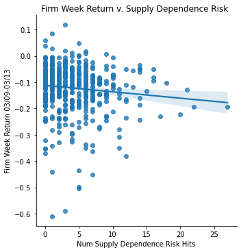
Measurement: Supply Dependence Risk
ret_v_supply = sns.lmplot(data=final_sample,
               x='Supply Risk', y='Weekly Return 03/09-03/13').set(
               title="Firm Week Return v. Supply Dependence Risk ",
               xlabel="Num Supply Dependence Risk Hits",
               ylabel="Firm Week Return 03/09-03/13")

ret_v_supply;
Regression Analysis for Supply Dependence
sm_ols('Q("Weekly Return 03/09-03/13") ~ Q("Supply Risk")',data = final_sample).fit().summary()
| Dep. Variable: | Q("Weekly Return 03/09-03/13") | R-squared: | 0.012 |
|---|---|---|---|
| Model: | OLS | Adj. R-squared: | 0.009 |
| Method: | Least Squares | F-statistic: | 5.657 |
| Date: | Fri, 25 Mar 2022 | Prob (F-statistic): | 0.0178 |
| Time: | 12:06:52 | Log-Likelihood: | 483.60 |
| No. Observations: | 488 | AIC: | -963.2 |
| Df Residuals: | 486 | BIC: | -954.8 |
| Df Model: | 1 | ||
| Covariance Type: | nonrobust |
| coef | std err | t | P>|t| | [0.025 | 0.975] | |
|---|---|---|---|---|---|---|
| Intercept | -0.1123 | 0.006 | -19.439 | 0.000 | -0.124 | -0.101 |
| Q("Supply Risk") | -0.0024 | 0.001 | -2.379 | 0.018 | -0.004 | -0.000 |
| Omnibus: | 172.409 | Durbin-Watson: | 2.136 |
|---|---|---|---|
| Prob(Omnibus): | 0.000 | Jarque-Bera (JB): | 662.686 |
| Skew: | -1.578 | Prob(JB): | 1.26e-144 |
| Kurtosis: | 7.758 | Cond. No. | 8.15 |
Notes:
[1] Standard Errors assume that the covariance matrix of the errors is correctly specified.
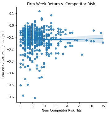
Measurement: Competitor Risk
ret_v_comp = sns.lmplot(data=final_sample,
               x='Competitor Risk', y='Weekly Return 03/09-03/13').set(
               title="Firm Week Return v. Competitor Risk ",
               xlabel="Num Competitor Risk Hits",
               ylabel="Firm Week Return 03/09-03/13")
ret_v_comp;
Regression Analysis for Competitor Risk
sm_ols('Q("Weekly Return 03/09-03/13") ~ Q("Competitor Risk")',data = final_sample).fit().summary()
| Dep. Variable: | Q("Weekly Return 03/09-03/13") | R-squared: | 0.000 |
|---|---|---|---|
| Model: | OLS | Adj. R-squared: | -0.002 |
| Method: | Least Squares | F-statistic: | 0.1401 |
| Date: | Fri, 25 Mar 2022 | Prob (F-statistic): | 0.708 |
| Time: | 12:06:53 | Log-Likelihood: | 480.84 |
| No. Observations: | 488 | AIC: | -957.7 |
| Df Residuals: | 486 | BIC: | -949.3 |
| Df Model: | 1 | ||
| Covariance Type: | nonrobust |
| coef | std err | t | P>|t| | [0.025 | 0.975] | |
|---|---|---|---|---|---|---|
| Intercept | -0.1240 | 0.007 | -18.682 | 0.000 | -0.137 | -0.111 |
| Q("Competitor Risk") | 0.0003 | 0.001 | 0.374 | 0.708 | -0.001 | 0.002 |
| Omnibus: | 166.003 | Durbin-Watson: | 2.111 |
|---|---|---|---|
| Prob(Omnibus): | 0.000 | Jarque-Bera (JB): | 602.293 |
| Skew: | -1.536 | Prob(JB): | 1.64e-131 |
| Kurtosis: | 7.492 | Cond. No. | 14.1 |
Notes:
[1] Standard Errors assume that the covariance matrix of the errors is correctly specified.
Measurement: Regulatory/Political Risk (all variations)
ret_v_reg1 = sns.lmplot(data=final_sample,
x='Regulatory Risk 1', y='Weekly Return 03/09-03/13').set(
title="Firm Week Return v. Regulatory Risk (1) ",
xlabel="Num Regulatory Risk (1) Hits",
ylabel="Firm Week Return 03/09-03/13")
ret_v_reg1;
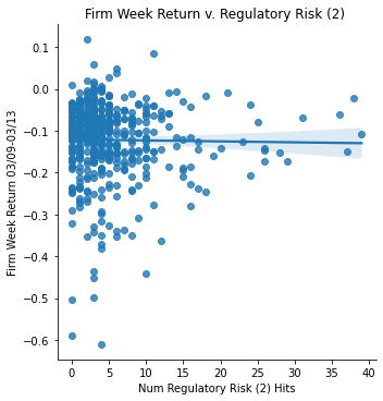
ret_v_reg2 = sns.lmplot(data=final_sample,
x='Regulatory Risk 2', y='Weekly Return 03/09-03/13').set(
title="Firm Week Return v. Regulatory Risk (2) ",
xlabel="Num Regulatory Risk (2) Hits",
ylabel="Firm Week Return 03/09-03/13")
ret_v_reg2;
ret_v_reg3 = sns.lmplot(data=final_sample,
x='Regulatory Risk 3', y='Weekly Return 03/09-03/13').set(
title="Firm Week Return v. Regulatory Risk (3) ",
xlabel="Num Regulatory Risk (3) Hits",
ylabel="Firm Week Return 03/09-03/13")
ret_v_reg3;


Regression Analysis for Regulatory Risk (1)
sm_ols('Q("Weekly Return 03/09-03/13") ~ Q("Regulatory Risk 1")',data = final_sample).fit().summary()
| Dep. Variable: | Q("Weekly Return 03/09-03/13") | R-squared: | 0.001 |
|---|---|---|---|
| Model: | OLS | Adj. R-squared: | -0.001 |
| Method: | Least Squares | F-statistic: | 0.3067 |
| Date: | Fri, 25 Mar 2022 | Prob (F-statistic): | 0.580 |
| Time: | 12:06:56 | Log-Likelihood: | 480.93 |
| No. Observations: | 488 | AIC: | -957.9 |
| Df Residuals: | 486 | BIC: | -949.5 |
| Df Model: | 1 | ||
| Covariance Type: | nonrobust |
| coef | std err | t | P>|t| | [0.025 | 0.975] | |
|---|---|---|---|---|---|---|
| Intercept | -0.1194 | 0.006 | -19.226 | 0.000 | -0.132 | -0.107 |
| Q("Regulatory Risk 1") | -0.0002 | 0.000 | -0.554 | 0.580 | -0.001 | 0.001 |
| Omnibus: | 168.798 | Durbin-Watson: | 2.118 |
|---|---|---|---|
| Prob(Omnibus): | 0.000 | Jarque-Bera (JB): | 627.751 |
| Skew: | -1.555 | Prob(JB): | 4.85e-137 |
| Kurtosis: | 7.605 | Cond. No. | 22.1 |
Notes:
[1] Standard Errors assume that the covariance matrix of the errors is correctly specified.
Risk Data vs. Return Analysis </br> Interestingly, none of my risk factors I measured had a strong negative or positive correlation with the returns from 03/09 to 03/24. However, certain risks had slight negative correlations. The most significant one was with Supply Dependence Risk. As shown with the regression analysis there is an intercept of -0.1123 (mostly negative returns) and a slope of-0.0024. It is expected that this should be a negative slope since firms with a more dependence on supply and supply chains would be disrupted during the initial outbreak of covid. However, I did expect there to be a steeper slope.
In regards to all of the regulatory variations and competitor risk data, they showed almost no, or very slight correlations with the return data. This means that having this type of risk did not really affect the firms differently when the pandemic hit. In contrast, I expected specifically the regulatory risk to have a negative correlation compared to the weekly returns.
Return Data vs. Other Firm Accounting Data:
This section will use the same type of analysis as presented before but will measure important accounting data to returns as opposed to risk data.
Measurement: PPE as a % of Assets
ret_v_ppe_a = sns.lmplot(data=final_sample,
               x='ppe_a', y='Weekly Return 03/09-03/13').set(
               title="Firm Week Return v. PPE as % of Assets",
               xlabel="PPE as a % of Assets",
               ylabel="Firm Week Return 03/09-03/13")

ret_v_ppe_a;

Measurement: Cash as a % of Assets
ret_v_cash_a = sns.lmplot(data=final_sample,
               x='cash_a', y='Weekly Return 03/09-03/13').set(
               title="Firm Week Return v. Cash as % of Assets",
               xlabel="Cash as a % of Assets",
               ylabel="Firm Week Return 03/09-03/13")
ret_v_cash_a;
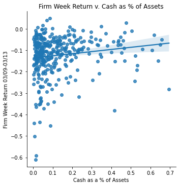
Accounting Data vs. Return Analysis </br> I isolated two different accounting data fields in order to see correlations with weekly returns. The first one was PPE as a percentage of Assets. As expected, there is a negative correlation between the two. When a firm has more PPE on hand, that means the firm has more leverage and thus will be more susceptible to economic impacts (if market does poor, these firms do really poor and vise versa). In contrary, there is a positive correlation between returns and cash as a % of assets. Firms with higher cash on hand did better during the initial covid outbreak, which also can be expected.
Return Data vs. Risk Values (Stimmy Day):
This section will use the same type of analysis as presented before but will measure the returns on 03/24 (stimulus day) as opposed to the previous 03/09 - 03/13.
#Read in the firm_returns dataset
firm_returns2 = pd.read_stata("2019-2020-stock_rets cleaned.dta")
firm_returns2 = firm_returns2[['date', 'ticker', 'ret']]

#restrict dataset to show specified dates only
firm_returns2 = firm_returns2[(firm_returns2['date'] == 20200324)]

firm_returns2['ret'] = pd.to_numeric(firm_returns2['ret']) #make the 'ret' column a numeric type
firm_returns2 = firm_returns2.assign(R = (1+firm_returns2['ret'])) #add new column 'R' which is simply 1 + 'ret' col

#group the dataset by ticker
firm_returns2 = firm_returns2.groupby(['ticker'])

#compute weekly firm returns for each firm
wkly_firm_returns2 = firm_returns2['R'].prod() - 1

#clean up DF
wkly_firm_returns2 = wkly_firm_returns2.to_frame() #convert series into DF
wkly_firm_returns2 = wkly_firm_returns2.rename(columns={'R': 'Weekly Return 03/24'})
wkly_firm_returns2 = wkly_firm_returns2.reset_index()

#merge sample_firms_risks into the weekly return DF to get one final DF
final_sample_stimmy = sample_firms_risks.merge(wkly_firm_returns2,
                        left_on='Symbol',
                        right_on='ticker',
                        how='left')

final_sample_stimmy = final_sample_stimmy.drop(['ticker'],axis=1)
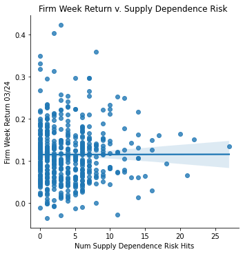
Measurement: Supply Dependence Risk
ret_v_supply_stimmy = sns.lmplot(data=final_sample_stimmy,
               x='Supply Risk', y='Weekly Return 03/24').set(
               title="Firm Week Return v. Supply Dependence Risk ",
               xlabel="Num Supply Dependence Risk Hits",
               ylabel="Firm Week Return 03/24")

ret_v_supply_stimmy;
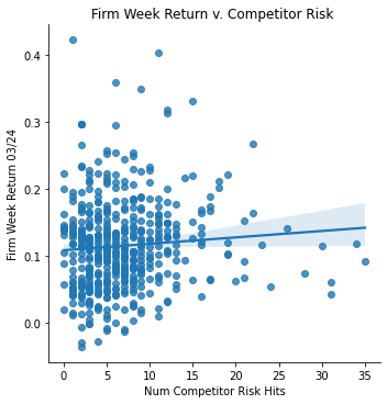
Measurement: Competitor Risk
ret_v_comp_stimmy = sns.lmplot(data=final_sample_stimmy,
               x='Competitor Risk', y='Weekly Return 03/24').set(
               title="Firm Week Return v. Competitor Risk ",
               xlabel="Num Competitor Risk Hits",
               ylabel="Firm Week Return 03/24")
ret_v_comp_stimmy;
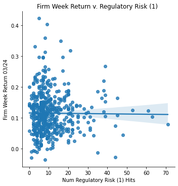
Measurement: Regulatory/Political Risk (1)
ret_v_reg1_stimmy = sns.lmplot(data=final_sample_stimmy,
               x='Regulatory Risk 1', y='Weekly Return 03/24').set(
               title="Firm Week Return v. Regulatory Risk (1) ",
               xlabel="Num Regulatory Risk (1) Hits",
               ylabel="Firm Week Return 03/24")
ret_v_reg1_stimmy;
Measurement: PPE as a % of Assets
ret_v_ppe_a_stimmy = sns.lmplot(data=final_sample_stimmy,
               x='ppe_a', y='Weekly Return 03/24').set(
               title="Firm Week Return v. PPE as % of Assets",
               xlabel="PPE as a % of Assets",
               ylabel="Firm Week Return 03/24")

ret_v_ppe_a_stimmy;
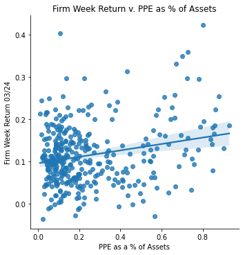
Stimmy Day Return Data Analysis </br> With stimulus day announced on March 24, 2020, the returns over that period skyrocked (comparatively to previous returns in that month due to covid). Every single firm in my dataset had a positive return on that day. Thus, when analyzing the returns vs. several risk measurements, it would be predictable of such correlation to be the opposite of what my previous correlations displayed.
Interestingly, this proved to be somewhat correct. The PPE vs. returns switched to a postive correlation, and the Competitor Risk vs. returns switched to be a slight positive correlation as well. However the supply dependence risk showed no correlation at all, likewise with the regulatory risk.